Authors: Compiled and organized by Daren Card with input from Anna Williford, Mehdi Eslamieh, Devendra Umbrajkar, Kevin Vilbig & Gaurav Kolekar.

License: GNU GPLv2

Adapted from: Software Carpentry, Data Carpentry, & Bruno Grande

Here are written lessons of the concepts taught at the UT-Arlington Software Carpentry workshop. These should provide enough details to allow you to essentially retake the course by yourself. Github can be used to make suggestions for improvements to these materials. We hope everyone found the workshop enjoyable and stimulating.

Before beginning, students should

1. Create a directory on their Desktop called ‘SCW_April2016’.
2. Download the zipped input files.
3. Unzip the download and move it into the ‘SCW_April2016’ directory.

Note: Users who completed the Git/GitHub portion of the workshop correctly should also be able to download their final output data.

Sections

Getting acquainted with the Bash shell environment

Analyzing and plotting data using Python

Establishing your online presence with Git and GitHub pages

Getting acquainted with the Bash shell environment

Motivation

The Unix shell has been in existence for decades and is therefore one of the most powerful pieces of software one can learn for data analysis. This is not only due to the fact it provides a powerful means of directly manipulating data. It can be used to write analysis scripts to automate data analysis. It is also the direct interface to most open-source software written for data analysis in the sciences. Therefore, even if you end up using Python or R for a lot of data analysis, you will also interact frequently with the Unix shell.

Overview of Lesson

Learners will explore the following concepts.

1. Using the Bash shell through the computer terminal.
2. Properly navigating through the computer file system hierarchy using the shell.
3. Creating, renaming, and deleting files and directories.
4. Manipulating text files to extract useful information.
5. Writing basic shell scripts to automate processes.
6. Working with multiple files at once using wildcards and loops.

Using the Bash shell

The Bash Shell may be new to most users and represents one of many command-line interfaces (CLIs) in use. It provides the ability to run programs and to write new programs. Apple and Linux users can access their Bash shell by opening the terminal and typing bash. Windows users will have to install and open git-bash.

Bash follows a Read-Evaluate-Print loop, meaning the computer reads input from the user, executes it, and prints the output of the process. The user provides the input at the prompt, which usually ends with $, which we’ve left out on all commands below. Let’s get familiar with this.

# '#' here and everywhere should be interpreted as comment

# echo command is executed: Try
$ echo "Welcome to our workshop"

# List of built-in bash commands:Try
$ help

# To get help for the command: Try
$ wc --help  
$ grep --help
$ man wc

# We will look at help pages in more details later
# And if you cannot find the command you want, google!

# TAB can be used to autocomplete accessible programs and directories/files.
# UP and DOWN arrows enable users to navigate through the history of commands they have run.

There are many commands natively available in the Bash Shell, most of which we won’t get to. You can use compgen -c command to list all the commands that are available on your system. Take a look at this cheat sheet to see more information on many of these.

As you can see from the list of Linux commands, bash can be used to deal with administrative tasks and text file manipulation, but it is also a programming language with variables, data structures, flow control statements and user-defined functions.

We will start by introducing simple administration-like commands that will allow you to find your way around the existing directory structure and then create new files and directories. After that we will see how to manipulate files and write shell scripts.

Navigate through your file system

Know who you are and where you are! Let’s talk about file system (folders and files) and how to find your way around.

# It can be useful to know which user you are on the computer. 
# Maybe not so much on your personal laptop, but definitely on public servers and other systems. 
# Use the following command to see the username of the active user.
whoami

As a long time user of computers, you’ve almost certainly become proficient in navigating your file system by clicking on folders and files using the GUI environment Desktop. You can do the same thing using the terminal.

# First, we should figure out where we currently are.
pwd  # stands for 'print working directory'
# Let's see what files and directories are available in our current working directory
ls   # stands for 'list'
# You can feed 'flags' or 'options' to many commands. 
# Using 'man <command>' in the Apple/Linux terminal will show these options (sorry, won't work on git-bash).
ls -F   # adds some extra info to the output, we will use this flag when we use 'ls'
# Another common task is simply moving through the file system to get to new locations.
# You should be starting out in your HOME directory, so typing the following will move you to your Desktop.
cd Desktop

Once you get used to the overall filesystem structure, which is pretty similar across operating systems and computers, you’ll be able to rapidly navigate to different locations. Take a look at this page for an overview on the basics of the typical Unix file system.

Challenge #1 Navigate to the folder you should have created before beginning this lesson. Once there, list the contents of the directory. Can you figure out how to list the contents without navigating to the folder?

Solution

# As separate commands
cd Desktop/SCW_April2016
ls -F
# As one command, from any directory
ls -F ~/Desktop/SCW_April2016

Absolute vs. Relative paths

So far, you have used what are called relative paths when moving between directories. This means that you have moved between directories based on your current location in the file system, or relative to your current location.

# You've seen how to move into a directory within your working directory.
# You can also move back out into the directory just outside of your working directory.
cd ..
# In this context '..' means 'the directory containing my working directory' or the parent of the current directory
# There is a similar notation for the working directory: '.'
# Let's list the contents of our current directory.
ls .
# One of the commands above also specified a directory relative to your HOME directory, which has '~' as a shortcut.
# Let's list the contents of our HOME directory.
ls ~
# Finally, sometimes it is useful to move back to your last working directory, whereever it is in the file system.
pwd
/Users/username/
cd Desktop/SCW_April2016
pwd
/Users/username/Desktop/SCW_April2016/
cd -
pwd
/Users/username/

Challenge #2 Make a diagram of the directory structure within HOME and practice navigation commands. The commands needed to do this are included above.

Creating, moving, and deleting files and directories

One of the major goals of any computer work is the create and remove directories and files. You can do the same very easily using the shell.

# Let's begin by moving into our 'SCW_April2016' directory
cd ~/Desktop/SCW_April2016
# Now let's make a single new directory called 'Linux'
mkdir Linux   # mkdir stands for 'make directory'
# If we wanted to immediately remove this directory, we could.
rmdir Linux   # rmdir stands for 'remove directory'... but let's not do this
# Create three move directories for each of the sections we will have in the workshop. You can do this w/ one command.
mkdir Python SQL Git
# You should now see these in your directory
ls
Linux  Python  SQL  Git
# Let's now move into the Linux directory and create an empty file.
cd Linux
touch MyFirstFile.txt   # touch simply initiates an empty file
# You can now add content using a text editor, which can be opened using the GUI or the terminal
edit MyFirstFile.txt  # this works on Apple, npp, subl, or other options exist depending on the platform.
# Be sure you save and close the editor in order to have your prompt return
# Now let's view the contents of the file.
cat MyFirstFile.txt   # cat stands for 'concatenate'

Files are commonly moved around in file systems, as you probably already know.

# renaming is accomplished by essentially moving a current file into a new file name.
ls
MyFirstFile.txt
mv MyFirstFile.txt MyFirstScript.sh  # syntax: mv $source $destination
ls
MyFirstScript.sh
# we can also move files between directories, which acts more like a conventional move.
# move our script to the Python directory
mv MyFirstScript.sh ../Python/
# check to make sure it works
ls
           # no files
ls ../Python
MyFirstScript.sh
# let's copy this back to our Linux directory
cp ../Python/MyFirstScript.sh ./
# This was a dummy file, so let's get rid of it
rm MyFirstScript.sh

Be careful when deleting files in the Bash Shell, as changes are final. There is no recycling/trash bin where you can recover it!

Challenge #3 We will soon be working with the files in the ‘data_linux’ directory you downloaded and unzipped earlier. It should currently be within the ‘SCW_April2016’ directory. Please move it to the ‘Linux’ directory to prepare fo the upcoming material. Also familiarize yourself with the contents of the ‘data_linux’ directory.

Solution

# This will work no matter where you are in your file system
mv ~/Desktop/SCW_April2016/data_linux ~/Desktop/SCW_April2016/Linux

Manipuating text files using the Bash Shell

Take a minute and open the ‘OECD_Countries_Full.txt’ file in Excel. You’ll see that this file contains some interesting information on many different countries in the world, including statistics on things like infant death rates, etc. We are going to spend some time manipulating this file to extract information using the Bash Shell. Some information you might want to know is:

1. How big is this file?
2. What countries does this dataset include?
3. What is the country with the highest infant mortality rate?
4. What country has lowest income inequality?
5. How do these countries rank with respect to taxes?
6. What year has the most data?

Let’s see how we can do some of this. But first create results folder in Linux folder. You now should have 2 folders in your Linux folder: data_linux and results. Change directory into results and let’s examine our data file.

# how large is your file `wc` outputs lines, words, bytes
wc OECD_Countries_Full.txt  # error! why? you should know why!
wc ../data_linux/OECD_Countries_Full.txt  # try also with absolute path!
# look at the first n lines
head -n 10 ../data_linux/OECD_Countries_Full.txt   # also try `tail`
# how many countries in this file?
cut -f1 ../data_linux/OECD_Countries_Full.txt
# you'll notice this prints the first column, country name, but there are lots of duplicates!
# we can redirect the output into a file, rather than as output in the terminal
# this is useful if we wanted to do more work using the output
cut -f1 ../data_linux/OECD_Countries_Full.txt > CountryList.txt
# view the contents of the output file
cat CountryList.txt
# in order to count the number of countries, we must combine two commands
# first we need to use 'sort' to sort the file so that all countries are clustered together on back-to-back (...) lines
sort CountryList.txt > SortCountryList.txt
# then we can use the 'uniq' to only output unique lines.
# uniq can only infer uniqueness if a file is sorted!
uniq SortCountryList.txt > UniqSortCountryList.txt
# and finally, we can use the familiar 'wc' command to count the number of lines, which is also the number of countries
wc -l UniqSortCountryList.txt   # -l (l as in lion) means only output 'lines'
# actually this number isn't totally correct, since it includes the header line, so we must subtract 1
# either way, this is a lot easier than counting by hand

Notice, we created 3 output files to find out how many countries are included into our dataset. You can fun ls to see for yourself. Do we really need them? One way to avoid generating intermediate files you do not need is to string different commands together, known as ‘piping’. Piping means that the output of one command is used as the input of the next command, which means it isn’t written to the disk. This is one of the most powerful aspects of the Bash Shell, which has been optimized over decades to facilitate just this type of data manipulation.

# the '|' (above the 'Enter' key) is used to perform piping
# we can perform the same analysis as above, start to finish, with 1 command!
# in this command the '-u' flag in 'sort' is the same as specifying 'uniq' separately
cut -f1 ../data_linux/OECD_Countries_Full.txt | sort -u | wc -l
# we can also add add another pipe to remove the "Country" header and get an accurate count
cut -f1 ../data_linux/OECD_Countries_Full.txt | sort -u | grep -v "Country" | wc -l

Challenge #4 Expand your piping skills by answering the following question. Which country had the highest “Infant_mortality” in 2012? Use OECD_Countries_Full.txt as an input file and generate CountryWithHighestMortality.txt as your ONLY output file. It is fine to generate intermediate files while you work towards a solution, but the ultimate solution should be only one command and output file~ You’ve seen all the commands necessary to perform this.

Solution

# begin by performing each step in the full pipe individually
# 1. select all rows with `Infant_mortality` in it
grep Infant_mortality ../data_linux/OECD_Countries_Full.txt > InfantMortality_all.txt
# 2. get data for 2012 only
grep 2012 InfantMortality_all.txt > InfantMortality_2012.txt
# 3. select only 1st and 6th columns
cut -f1,6 InfantMortality_2012.txt > InfantMortality_2012_short.txt
# 4. sort by 2nd column from min to max
sort -n -k2 InfantMortality_2012_short.txt > InfantMortality_2012_short_Sorted.txt
# 5. select country with highest mortality rate
tail -n 1 InfantMortality_2012_short_Sorted.txt > InfantMortality_2012_short_Sorted_Highest.txt
# now let's put this together into single piped command, as instructed
grep Infant_mortality ../data_linux/OECD_Countries_Full.txt| grep 2012 | cut -f1,6 | sort -n -k2 | tail -n 1 > CountryWithHighestMortality.txt 

Constructing Shell scripts for automation

But what if you want to reuse these commands? You want to do something similar on another file? We need to save the commands to file so we can easily reuse/modify them later. Such collection of commands in the order you want them to be executed is a simple shell script.

Let’s make scripts folder in the Linux folder. Go to scripts. We will keep our scrpts here. While in results folder you can mkdir ../scripts

# copy and paste or just redirect the line that works (from history) to `MyFirstScript.sh` file
# echo simply echos the text you provide back to the terminal as output, much like printing
$ echo "grep Infant_mortality ../data_linux/OECD_Countries_Full.txt | grep 2012 | cut -f1,6 | sort -n -k2 | tail -n 1  > CountryWithHighestMortality.txt" > ../scripts/MyFirstScript.sh

Notice we created MyFirstScript.sh in script directory. Let’s view and modify it slightly. You can view it from your current directory or cd into scripts and view from there using your favorite text editor. Examples: npp MyFirstScript.sh or edit MyFirstScript.sh.

We’ll add three lines at the top of the file

1. The shell that should be used to execute your code: #!/bin/bash
2. A one-line description of what your script does
3. Usage statement so people can determine how to run your script: usage: MyFirstScript.sh

Let’s run it from scripts directory. But first look at it carefully, do you think it will run?

#./ indicates that you are running script from working directory
./MyFirstScript.sh

But is it a good script? Would it run from any directory? Could you reuse with a different file? How can we make it more flexible?

To make it flexible we need to introduce a variable for a part of code that we want to change frequently. Variables store values like they do in mathametics. For example, if we want to run this code with a different file, we want a variable instead of hard-wired filename; a variable can take any user-defined value.

# here is a quick examples of variables using the Bash shell
myname=Name
echo Name
Name
echo myname
myname       # not what we want!
echo $myname
Name	     # the '$' before makes something a variable!

Let’s modify MyFirstScript.sh to include a variable and save it as ‘MyFirstScript_Variable.sh’.

Here is MyFirstScript_Variable.sh

#!/bin/bash

# record a country with highest Infant_mortality among countries in OECD_Countries_Full.txt
#usage: script.sh

input=../data_linux/OECD_Countries_Full.txt

grep Infant_mortality $input | grep 2012 | cut -f1,6 | sort -n -k2 | tail -n 1  > CountryWithHighestMortality.txt

Run it from scripts: ./MyFirstScript_Variable.sh

Is it better? A little bit. Hopefully you see why. What would be even better? We probably want to provide filename at the command line and not have to change the script itself. Let’s create a new script called ‘MyFirstScript_NaiveVariable.sh’.

Here is MyFirstScript_NaiveVariable.sh

#!/bin/bash

# record a country with highest Infant_mortality among countries in OECD_Countries_Full.txt
# usage: script.sh $inputFile   #notice how we need to run this now

input=$1  #special variable that stores the the first argument at the command line

grep Infant_mortality $input| grep 2012  | cut -f1,6 | sort -n -k2 | tail -n 1  > CountryWithHighestMortality.txt

Run it from scripts: ./MyFirstScript_NaiveVariable.sh ../data_linux/OECD_Countries_Full.txt

This script is much better, but it can certainly be even better!

Challenge #5 Work in groups to write a script that would allow user to compare any indices between the countries (not just Infant_mortality), use data for any year (not just 2012) and write the output to a user-defined output file.

Solution Here is MyAwesomeFirstScript.sh

#!/bin/bash

#record a country with highest Infant_mortality among countries in OECD_Countries_Full.txt
#usage: script.sh $inputFile $index $year $outFile   #notice how we need to run this now

input=$1              #special variable that stores the the first argument at the command line
measure=$2            # $2, $3, $3 store values from 2-4 command line arguments
year=$3
out=$4

grep $measure $input| grep $year| cut -f1,6 | sort -n -k2 | tail -n 1  > $out

Run it from scripts: ./MyFirstScript_Good.sh ../data_linux/OECD_Countries_Full.txt Income_inequality_interdecile_ratio_P90_P10,_level,_late_2000s 2013 CountryWithHighestIncomeInequality.txt

This is much better. If you want to keep output files in results folder, your output file should be ../results/CountryWithHighestIncomeInequality.txt

Working with multiple files at once using wildcards and loops

Go to data_linux/ByCountry. This directory contains data from OECD_Countries_Full.txt but was split by country using this command: grep -v Country OECD_Countries_Full.txt | awk '{print >$1"_data.txt"}'. If you stick with this, one day you will understand this command!

We can use a wild card to get information about multiple files at the same time, instead of issuing commands for each file, one at a time.

# the '*' wildcard matches any anything, whether a single character or many
wc -l *     # print number of lines for all files
# we can restrict our wildcards a little
# let's only print the number of lines for those files that start with 'A'.
wc -l A*
# we can instead print the number of lines for files that start with 'I' and have an 'e' somewhere inside the file.
wc -l I*e*
# the '?' wildcard matches a single instance of something
# we can print the number of lines for files that start with 'I' and have an 'e' as the 3rd character.
wc -l I?e*

These are the simplest forms of what we call regular expressions. These get way too complex for this lesson, but you can find out more by about how powerful regular expressions are.

The wc command knows to operate on each file when you provide a wildcard. However, some commands cannot do this, like the script we created before. In these cases, we have to run a commmand on multiple files using a loop.

# here is a very simple loop that will echo (print) the name of each file in your working directory
for file in *; do echo $file; done

Let’s use this loop idea to run a script that will extract data on particular measure from every country file found in ByCountry folder and record it to a single output file

This is CollectDataFromByCountry.sh. Save it to ByCountry folder for now.

#!/bin/bash
# this script collects data of user-specified index measured in a given year from all country-specific files
# usage: script.sh $inputFile $measure $year

input=$1
index=$2
year=$3

# note the '>>'. This means append instead of write, so that the output won't overwrite previous output.
grep $index $input| grep $year | cut -f1,6 >> $index"_"$year.txt 

Now that we have a command we want to run on each file in ‘EveryCountry’, we must put it into a loop.

# let's extract the lies from each file that contain the 'Total_fertility_rates' from 2012
for file in *; do CollectDataFromByCountry.sh $file Total_fertility_rates 2012; done 
# now we should see a file called 'Total_fertility_rates_2012.txt' in the 'EveryCountry' directory.

Challenge For you final challange, go to ByMeasure directory. In this case the files contain data from OECD_Countries_Full.txt but was split by measure/index using this command: grep -v Country OECD_Countries_Full.txt | awk '{print >$3"_data.txt"}'

Take a look at a file to see what this command did. Now write a script that will collect information from every measure-specific file for a user-defined country. Hint: This will be very similar to the script we’ve already worked with.

Once your script is complete, use a loop to run it on each file in the ‘ByMeasure’ directory.

Solution This is GetCountryInfo.sh. Save it to ByMeasure folder for now.

#!/bin/bash
# this script collects data for user-specified country from all index-specific files
# usage: script.sh $inputFile $country

input=$1
country=$2

grep $country $input >> $country.txt 

Run it from ByCountry folder:

for file in *; do ./GetCountryInfo.sh $file Sweden; done 

Additional Resources

• Linux OS:
  • http://www.linfo.org/
  • http://www.tutorialspoint.com//operating_system/os_linux.htm
• Linux servers
  • UTA: omega, HPC
  • TACC
• Linux commands
  • http://linuxcommand.org/
  • http://cli.learncodethehardway.org/bash_cheat_sheet.pdf
  • http://www.pixelbeat.org/cmdline.html
  • http://ss64.com/bash/
  • https://linuxconfig.org/linux-commands
• Linux file/directory naming rules
  • http://www.cyberciti.biz/faq/linuxunix-rules-for-naming-file-and-directory-names/
• Bash scpipting titorial
  • https://linuxconfig.org/bash-scripting-tutorial

Analyzing and plotting data using Python

Motivation

Python has emerged as one of the premier frameworks for data manipulation and analysis in recent years to to its easy-to-read syntax, speed, and great community support. As such, it is also becoming the go-to introductory programming language in many learning settings. Given its relative youth, it is likely Python will continue to overtake alternative programming languages for a variety of reasons.

Overview of Lesson

Learners will explore the following concepts.

1. Important data analysis packages for use in Python.
2. Reading common text formats.
3. Gathering basic information and statistics from tabular data.
4. Making basic plots of data.

Important necessary packages into Python

Python relies on packages to provide useful functions to users. Therefore, when one begins using Python, he or she must tell Python to import the necessary packages to complete the given work. For this portion of the lesson, we will be working with the packages sys, matplotlib, and pandas.

# packages import syntax: import <package> or from <package> import *
# users can also import to a variable, which can be useful: import <package> as <variable>
import matplotlib.pyplot as plt
import pandas as pd               #this is how I usually import pandas
import sys                        #only needed to determine Python version number
import matplotlib                 #only needed to determine Matplotlib version number
from pandas import *
%matplotlib inline                #Enable inline plotting

Packages will be periodically updated, so it is important to be able to keep track of package versions. Sometimes certain functions will be limited or unavailable in certain versions.

# let's check what version of pandas we are using
# note that we read pandas in as 'pd' to save a bit of typing
pd.__version__

Reading data for use in Python

Python provides many useful commands for reading and writing text files, as this is the first and last step, respectively, in any successful data analysis. Common text formats for tabular data are comma-separated values (csv) and tab-separated values (tsv), and you can commonly tell which is which by looking at file extensions. Let’s create a series of commands to read in a tsv file and write out a csv.

import csv      # A useful package for readin tablular data

# remember that tsv is input and csv is output
# if working on Mac/Linux, the below absolute paths will be different, so adjust accordingly
# set variables for the input and output files, called tsv_file and csv_file respectively
tsv_file = "C:/Users/MMEslamieh/Desktop/SCW/OECD_data_25Countries_Full.tsv"
csv_file = "C:/Users/MMEslamieh/Desktop/SCW/OECD_data_25Countries_Full.csv"

# read the input file to a object called 'in_tsv', specifying tab-delimited ('\t') values
in_tsv = csv.reader(open(tsv_file, 'r'), delimiter = '\t')

# initalize an empty output file to write to
out_csv = csv.writer(open(csv_file, 'w'))

# create a for loop that reads each line from the input tsv file
# and writes it to an output csv file
for row in in_tsv:
    out_csv.writerows(in_txt) 
    
# close the output file to finish writing
out_csv.close()

Gathering some basic information about our data

Now let’s start from scratch, to a degree, by reading in a our tabular data using pandas, which is designed for this type of data.

# let's read our working data in again using pandas
data = pd.read_csv('Desktop/SCW/Test/OECD_data_25Countries_Full.csv')

# now we can gather a basic understanding of our data using a few commands
data.head()                      # show first five rows-default
data.head(10)                    # show first ten rows
data.tail()                      # show last five rows
data.info()                      # summary of data
data.Year.value_counts()         # Count the number of Values
data.describe()			 # description statistics of data frame
data.GNI.describe()		 # description statistics of single column: GNI
data.ix[2:4,['Country', 'GNI']]  # slicing by row and column
data['GNI'].max()		 # or data.GNI.max(), maximum of GNI column
data['GNI'].min()		 # or data.GNI.min(), minimum of GNI column
data['GNI'].median()		 # or data.GNI.median(), median of GNI column
Year2011 = data[data.Year==2011] # filter for specific column, storing as an object
Year2011.sort_index()            # sort our stored object by row
Year2011.sort_index(axis = 1)    # sort our stored object by column
Sorted_2010 = Year2010.sort_index(ascending=[False,True], by=['GNI','InfantMortality'])   # sort by two columns, storing as an object
Year2011.to_csv('Desktop/SCW/Test/Year2011.csv') # save 'Year2011' object as CSV format

Subsetting and grouping data

With tabular data, sometimes multiple rows may contain the same value in a given column. One may want to calculate statistics on only those rows that can be grouped together by a certain column. For example, given the data we are working with, someone may want to determine the average infant mortality rate across countries in the year 2012.

data_grouped = data.groupby('Year')  	 # group the Year 
data_grouped.GNI.median()            	 # Show the median of each group(country) separately
data_grouped.GNI.describe()		 # summary statistics
data_grouped.get_group(2011).GNI.hist()  # make a histogram of 2011 only
data_grouped.get_group(2012).GNI.hist()  # run with above line make two histogram simultaneously, side by side plot
data_grouped.boxplot(column = 'GNI')     # compare boxplots side by side

Creating plots of data for visualization

We’ve seen a few basic plots above, but it is definitely worth devoting a whole section to plotting.

# create a histogram
data.GNI.hist() 
data.GNI.hist(bins=20) 			# set the number of bins for histogram
# create an area plot
data.IncomeInequality.plot.area()
# create a box plot
data.boxplot(column='GNI')
# now let's make a plot and manipulate some attributes like color
data['GNI'].plot()        		# or data.GNI.plot()
data.plot(x = 'Country', y = 'GNI', color = 'red', figsize =(20,5), kind = 'bar')

Challenge #1 Spend a few minutes making plots of various columns in our data. Try adjusting options like the color, plot size, and plot type. You can use Google to try to experiment with other options.

One can also create plots by adding successive layers, like below.

# create a plot object with a basic plot, like that we've alrady made
d = data.plot(x = 'Country', y = 'GNI', kind = 'bar', color = 'red' , figsize= (20,5))
# now we can add things like labels and legends
d.set_title ('GNI over country' , fontsize =40) # Add the title to the plot
d.set_xlabel('Country',fontsize =20) 		# label the x axis
d.set_ylabel('GNI',fontsize =20) 		# label the Y axis
d.legend(['Test']) 				# Legend the plot
# we can now save our figure
fig = d.get_figure()                		# Gather the figure as object 'fig'
fig.savefig('Desktop/SCW/Test/Year_2011.png')	# Write out

Now let’s create a scatter plot and view the correlation between a couple of our columns.

# let's just work with the year 2011, using an object we already created
d = data_2011.plot(kind = 'scatter', x ='InfantMortality' , y ='IncomeInequality', color = 'green', figsize = (20,5), marker = '*', s = 100)
d.set_title ('Year 2011', fontsize = 40)
d.set_xlabel('Infant Mortality',fontsize = 20)
d.set_ylabel('Income Inequality',fontsize = 20)
d.legend(['Test'])
# now calculate the correlation between these fields
slope = data_2011['IncomeInequality'].corr(data_2011['InfantMortality'])
slope

Additional Resources

• pandas
  • http://pandas.pydata.org/
  • https://pypi.python.org/pypi/pandas/

Establishing your online presence with Git and GitHub pages

Motivation

It is becoming evermore important to establish a web presence, even as an undergraduate student. Facebook, Twitter, and the like are methods for doing this, but many would agree that it is much more professional to give people a snazzy website. Historically, people gravitated towards large website creation websites or had to learn HTML and other languages to build their own websites. Then there was the arduous task of finding or paying someone to host your website. Fortunately, the increased expectation of creating and maintaining a website is correlated with the increased ease in doing so, due in part to cloud-based hosting solutions and intuitive markdown-based methods of building content.

GitHub has emerged as one of the best options creating an awesome looking website easily and cheaply (even free!). As the name implies, GitHub was founded as simply a online hub, or hosting service, for Gits, or as they are commonly called, Git repositories. Git, put simply, is a flexible and powerful file management and archival system. It was built with complex project management in mind, in an effort allow project developers to keep track of file identities and versions, and seamlessly navigate through this complex temporal and hierarchical file-system structures. If this isn’t making sense, the comic below more-or-less outlines what Git allows users to avoid.

Overview of Lesson

Learners will complete the following broad tasks:

1. Fork a website template repository on GitHub and use Git locally to pull this repository onto their computer.
2. Make necessary changes to setup the website and then add content, using Markdown, while learning the basics of Git.
3. Push local changes back to remote repository at GitHub, which then automatically builds and displays the website.
4. Users will conclude by populating their website with all materials and overviews of the lessons for the Software Carpentry workshop they participated in. This will allow them to reference this information later.

Forking and Cloning a Repository

GitHub Pages, GitHub’s service that builds and hosts websites, utilizes several fairly complex programming languages, thus saving the user the trouble of knowing them in great depth. One simply has to provide a properly formatted repository and GitHub does the rest. We will take advantage of this, plus open source website templates, to create personal websites. For this lesson, learners will be using the Jekyll Now template, but there are many options out there.

This template is contained in a repository owned by Daren Card, which is modified slightly from its original form. It was originally created by Barry Clark. This means that we cannot edit it ourselves. Rather, we will be creating our own copy of it and then modifying it to our liking. The copying will take place on GitHub using a process called ‘forking’ and the editing will take place using a simple text editor on the user’s local computer. Visit the modified Jekyll Now template repository from Daren and click the Fork button at the top-right. If you happen to already be affiliated with another organization in GitHub, you may be prompted to select an account, and you should use your personal GitHub account.

We’ll make some pretty basic changes online to the repository settings. Under the top tabs is a brief description of the repository that we inherited as part of this template. Click to edit and give your repository a new, brief description. Also include the URL we will use to access your forthcoming website, which should be <username>.github.io, where <username> reflects your GitHub username.

From here, we will work further on our repository on our local computer. Before doing so, we must setup Git for the first time on our machine.

# setup the name git will call us by
git config --global user.name "First Last"
# setup the email address to use. must match that used to create github account.
git config --global user.email "email@domain.com"
# add some useful colors to output
git config --global color.ui "auto"
# specify text editor, to be used in committing. Choose appropriate option:
# nano: git config --global core.editor "nano -w"
# text wrangler: git config --global core.editor "edit -w"
# notepad++: git config --global core.editor "'c:/program files (x86)/Notepad++/notepad++.exe' -multiInst -notabbar -nosession -noPlugin"
# kate: git config --global core.editor "kate"
git config --global core.editor "<choice">
# now take a look at these settings (and more)
git config --list

To work locally, we must download the repository from GitHub, which is called ‘cloning’. We can do this as a zipped file, but let’s instead learn our first bit of Git. Along the top of your files list you should see a URL. Be sure that the box to the left reads ‘HTTPS’ and not ‘SSH’. The latter requires some further steps, that we will leave that for you to do later using instructions on setting up SSH keys. Copy the HTTPS link and in your Terminal type the following commands.

# Create a 'Repos' directory in your $HOME folder
mkdir -p ~/Repos
# Change into your new directory
cd ~/Repos
# Clone your website template repository from GitHub
git clone https://github.com/<username>/<username>.github.io.git

You should now see a see a local copy of your repository in the working directory.

Exploring Git

We should now spend some time explaining Git in more detail.

# Change into your repository directory and view its contents
cd <username>.github.io
ls

You should see the same exact list of files that was observed on GitHub. So what makes this a Git repository? It appears to be like any other directory. Let’s explore that question.

# List the full contents of the directory, including hidden files, as a single column
ls -1a
.
..
.git
.gitignore
404.md

You should now notice several files with leading dots, indicating they are hidden. The first and second represent the working and upper-level directories, respectively. The next ‘.git’ file is the key to a Git repository, as it contains the information that Git (and GitHub, which is essentially Git running on a server, with some fancy add-ons) use to manage this directory as a repository.

We’ve copied this directory, so let’s take a quick tangent and explain how one would initialize a Git repository in any directory.

# Change directory to the upper-level (notice the use of the ..)
cd ..
# Make a new directory called whatever you want (I'm using 'biology') and move into it
mkdir biology
cd biology
# Create some empty files/directories to make this appear like a normal directory
mkdir genetics ecology microbiology
touch zoology botany

So now we have essentially the same thing as our copied website template, but without the ‘fancy’ Git hidden files. Let’s create those now.

# Initialize your directory as a Git repository
git init
# View the directory contents
ls -1a
.
..
.git
botany

So we now have the the .git hidden file, but what about that .gitignore one. All the .gitignore file specifies are the files and/or directories that you want Git to ignore when it tracks the files in your repository. Therefore, if we find plants boring (because they are!), we could have Git ignore the ‘botany’ file. We do this by simply adding the names of the files/directories we want to ignore.

# One way of adding 'botany' to our gitignore, sans text editor
echo 'botany' > .gitignore

That gives some basic Git information, and we’ll explore more with real files inside of our website repository.

Setting Up Your Website

We’ll begin by configuring a couple files that establish the overall website design and that tell our visitors some basic information about ourselves. Let’s first edit the _config.yml file to set some overall design parameters. Open this file in a text editor and fill in some basic information.

name: <name>
description: <name>'s website
url: <username>.github.io

Let’s also replace that stock photo with something more personal. Go online and find a picture of yourself, or of something fitting of yourself (that you have permission to use). In many cases, you can right-click and select “Copy Image URL” or something similar. If your lazy you can just use your GitHub image. You can place this as your avatar.

avatar: http://domain.extension/images/picture.jpg

Now let’s edit the ‘About’ page on our website and provide any visitors with basic information about yourself. When you open the file in a text editor, you’ll see the following header. It simply specifies information about the page design, title, and relative link.

---
layout: page
title: About
permalink: /about/
---

Next you can modify the text accordingly to tell people about yourself. Notice the pound signs at the beginning of a couple lines and how they translate to the relative text rendering on the website. The syntax is called Markdown and it allows us to take simple text and add some flare without a bunch of coding knowledge. This lesson overview is written in markdown as well. You can use the brief guide at GitHub to get a feel for Markdown.

Integrating Our Changes and Visualizing the Results

Now we want to see what our changes have done to the website. This will introduce the most commonly used Git commands. Let’s start by viewing our Git status.

git status
On branch master
Your branch is up-to-date with 'origin/master'.
Changes not staged for commit:
  (use "git add <file>..." to update what will be committed)
  (use "git checkout -- <file>..." to discard changes in working directory)

	modified:   _config.yml
	modified:   about.md

no changes added to commit (use "git add" and/or "git commit -a")

The output provides us with some useful information, like the branch name (something we won’t really discuss today). It also includes our two modified files and tells you that neither have been added to commit. Let’s progress by both adding and committing the changes we’ve made. You should also view the Git status after each one.

git add _config.yml about.md
# Hopefully you are noticing the intuitive verbs that Git uses
# This one adds your files to Git's tracking
git commit -m "added some basic website info"
# This command commits your changes and provides a useful message about what they are

You can also view your Git log and see info on the changes you’ve just made, including obvious things and also a computer generated label for the commit (that long alphanumeric string).

git log
commit a69c34a76c0fa85b7ffc86237fb34c8e0f6ae4c3
Author: darencard <dcard@uta.edu>
Date:   Fri Jan 22 22:43:55 2016 -0600

    added some basic website info

The steps you just took made your first Git commit, so Git has recorded these initial changes. Let’s make some more quick changes to your _config.yml. You’ll notice that there are fields like ‘email’ and ‘github’ (and others) where you can include your email address and GitHub handle for people to interact with you. Fill one or two in.

Another key attribute of Git is that it allows you to compare versions of files and note differences. Let’s compare our _config.yml file from our two commits.

git diff
diff --git a/_config.yml b/_config.yml
index b89b129..5a4572f 100644
--- a/_config.yml
+++ b/_config.yml
@@ -21,12 +21,12 @@ footer-links:
   email:
   facebook:
   flickr:
-  github:
+  github: darencard
   instagram:
   linkedin:
   pinterest:
   rss: # just type anything here for a working RSS icon
-  twitter:
+  twitter: darencard
   stackoverflow: # your stackoverflow profile, e.g. "users/50476/bart-kiers"
   youtube: # channel/<your_long_string> or user/<user-name>
   googleplus: # anything in your profile username that comes after plus.google.com/

As you can see, Git gives you pretty intuitive information on the files being compared (plus abbreviated labels) and the specific changes made to the file. Now go ahead and practice adding and committing your new changes. If you view your log again you’ll see this second commit.

Now let’s say that you made a mistake in editing the _config.yml file. In this context, it would be very easy to open the file back up and make a couple quick edits. However, what if this file is much more complex, like a long shell script, or what if you go through a series of edits and still have an error, and just want to revert to the last working version you had. Git allows you to do this.

# Revert to the previous commit
git checkout HEAD~1 _config.yml
# Revert to the commit before the previous commit (or beyond)
git checkout HEAD~2 _config.yml
# Revert to a specific commit using the full commit label
git checkout a69c34a76c0fa85b7ffc86237fb34c8e0f6ae4c3

You can use similar relative or absolute commit syntax to compare committed files using a command we’ve already seen.

# Compare two previous commits
git diff HEAD~1 HEAD~2 _config.yml
# Compare our newly edited, uncommited files to an exact commit by label
git diff a69c34a76c0fa85b7ffc86237fb34c8e0f6ae4c3

Integrating Our Changes with our Website

These previous steps demonstrate the basics of Git, which can be used locally to keep track of changes to files without having to make separate file copies for each change. Let’s take this full circle and reintegrate our changes remotely, on GitHub’s servers, and thus customize our website.

# Let's make sure we are at the head of our branch
git checkout HEAD
# Push our changes to GitHub where it can be integrated into our website
# 'origin' refers to the remote server and 'master' to the branch
git push origin master
Counting objects: 7, done.
Delta compression using up to 4 threads.
Compressing objects: 100% (7/7), done.
Writing objects: 100% (7/7), 585 bytes | 0 bytes/s, done.
Total 7 (delta 5), reused 0 (delta 0)
To https://github.com/darencard/darencard.github.io
   0ed1225..84634d5  master -> master

Now if we refresh our GitHub repository page we should see the changes, including the commit messages. You can click on these files and view their contents, and you can even compare versions within GitHub, just like we’ve already done locally. Now view your website using your URL and you’ll see the changes reflected (sometimes GitHub takes a few minutes to render changes).

Populating Your Website with Workshop Content

Part of the goal of this exercise, especially during a workshop, is to provide the learner with a compact package containing everything they need to go through the workshop again or to refresh their memory. Distributing this package in the form of a website repository not only provides all the files the user needs, but also allows the user to visualize the lessons from anywhere at anytime through a static website. If you look at the repository you originally forked, you’ll see it contains the raw data that was used for the other portions of the Software Carpentry workshop attended. It also contains the markdown files with the lesson overviews (which you are currently reading). Unfortunately, the repository does not contain the output files generated as part of the workshop, which may be beneficial to have if one wants make comparisons with later work.

Let’s begin by creating a .zip archive containing the output from the other portions of the workshop.

# Copy all output into a new directory 'output_data'
# It would probably be best to organize files into subdirectories for Linux, Python, SQL
# Zip the output_data directory
zip -r output_data.zip output
# Move output_data.zip into the 'data' directory of your website repository

Now we can add, commit, and push these changes.

git add *
git commit -m "Added output zip"
git push origin master

Now if we look at our website, we can view all of the lesson writeups, complete with both the raw and output data.

Using a Pull Request to Help a Friend

Let’s say that you have a friend who also took the Software Carpentry workshop, but who had to leave a little bit early. Therefore, he or she didn’t get a chance to properly add the output data to their website repository and has since deleted it. They ask you to help them out. Normally, one may just email the file over, but GitHub offers an alternative method of getting this data to your friend, with the added benefit of placing it directly into the correct location within your friend’s repository. This method is called a Pull Request.

To perform a Pull Request, you must first navigate to your friend’s website repository. Click the ‘New pull request’ button above the file list.

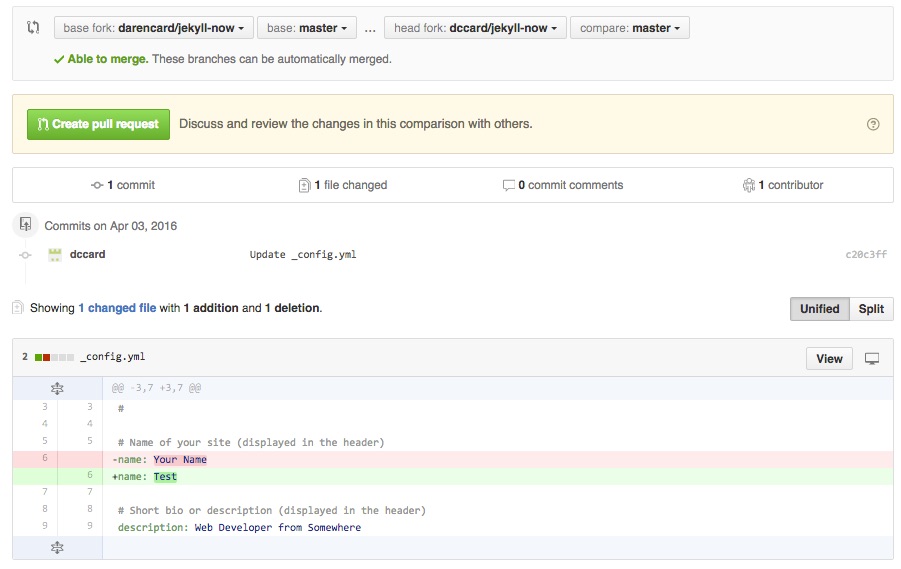
On the next page you will see a few pieces of important information. The bar along the top displays the forks and branches that are to be merged. The ‘base fork’ should be your friend’s repository where you are trying to send your updates. The ‘base’ refers to the branch on that repository you are merging too, which will almost always be ‘master’. The ‘head fork’ is your updated repository with the changes you are trying to send to your friend. In this case, you are comparing your ‘master’ branch with your friend’s repository. Below you will see information on the number of updated commits and files, information that should match your expectations. When working with text files, like scripts, you should also see an intuitive graphic showing the change, with subtractions indicated in red with a ‘-‘ sign and additions indicated in green with a ‘+’ sign. Github makes some checks to be sure that you can merge these forks together (see “Able to merge” in the above bar, but you should use this page to make sure you are happy with the changes you are sending to your friend’s repository. Once satisfied, you can press the ‘Create pull request’ button near the top of the page.

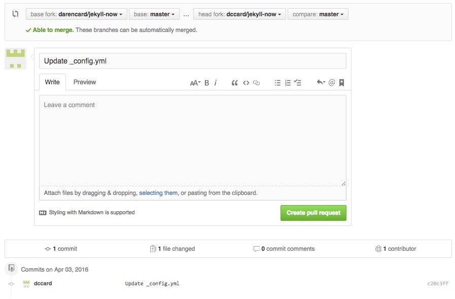
On the next page you will see a text box with a subject line, much like an email message. This is what you use to provide information on the Pull Request you are undertaking, so that the other use can easily know the basics of what you are contributing. In the subject/header line you should write a brief, but informative, phrase about the changes occurring. If you would like to add more information, you can use the large text block below to provide more details. In this text block, it is possible to use markdown to render your information, and you can use the preview button to see what this will look like. Take a minute to create an informative message and comment to your friend and click ‘Create pull request’ near the bottom of the page.

Finally, you will see a confirmation/summary page about the Pull Request you just completed. GitHub again gives you the option of leaving a comment to help others understand your changes.

Before your changes can be incorporated, your friend must actually ‘Merge’ your Pull Request. He or she must log into his or her account and should see a notification that a Pull Request is pending. This will take your friend to a page like that below, where he or she can view the changes you propoed.

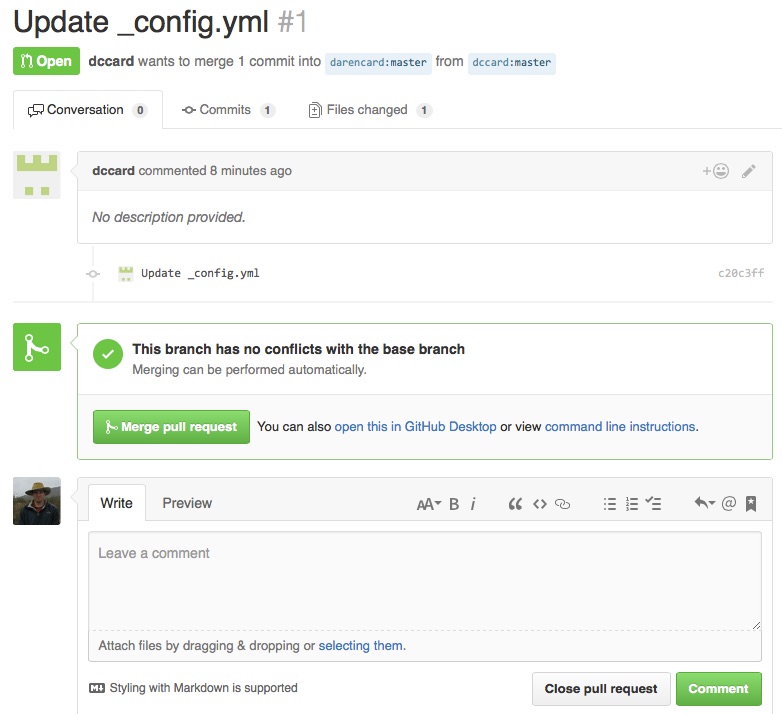
The ‘Conversation’ tab contains the description of the pull request you gave when you created it, and users can use this space to converse about potential changes over a series of messages, if needed. The ‘Commits’ and ‘Files changed’ tabs are can be used to view the commits made and the actual file changes, using an environment that is similar to what you interacted with during your Pull Reqeust. When your friend is satisfied that he or she wants to accept your Pull Request, he or she can click ‘Merge pull request’. If the changes aren’t appropriate after some conversation, he or she can instead click ‘Close pull request’. Upon accepting a pull request, your changed file(s) will be incorporated into your friend’s repository, and his or her website should update to reflect the changes. Basically, your friend’s website will now contain an active link to the output data that he or she was missing.

Additional Resources

• Git/GitHub
  • Software Carpentry
• GitHub Pages
  • GitHub Guide